x <- 5
y <- "string"
x*2
[1] 10print(y)[1] "string"Course website: https://hannahmetzler.eu/R_intro/
x <- 5
y <- "string"
x*2[1] 10print(y)[1] "string"rm(list = ls())rnorm(20, mean = 100, sd = 10) [1] 93.93979 104.74322 96.06165 104.73950 99.44939 83.59975 109.45312
[8] 89.81305 114.86397 109.16977 93.64867 97.76352 110.52766 79.01328
[15] 82.58372 108.11045 98.70091 94.06051 100.47008 94.43081?rnorm# install.packages("tidyverse")
library(ggplot2)
library(dplyr)
library(readr)Before we create our first R-project, we need to talk about how to name files and folders, and how the file system and file paths on your PC work, and how you navigate your way through it.
data_file.csv_) to separate parts of the file name, and dashes (-) to separate words in a section "data_questionnaire_2021-11-15.xls"Data (Participants) 11-15.xlsfinal report2.docParticipants Data Nov 12.xlsproject notes.txtQuestionnaire Data November 15.xlsreport final.docreport final 2.doc_project-notes.txtdata_participants_2021-11-12.xlsdata_participants_2021-11-15.xlsreport_v1.docreport_v2.docreport_v3.docdirectory/subdirectory/
/Users/UserName/, or on Windows: C:\Users\Username\/Users/UserName/Desktop/datafile.csvCommand Prompt - it won’t work in the same way.
bash.bash, so make sure you get them all right!bash, you can use these commands to navigate between folders:
cd change directory, e.g., to move to my user directory: cd /Users/Hannah/~ shortcut for the user account directory `/Users/UserName/, e.g., to move to the user directory: cd ~.. move one directory upwards: cd ..cd. In R, we would have () instead: function()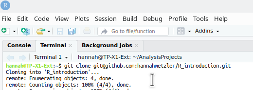
I find it useful to have all my analysis projects in a common folder directly in my user directory: ~/AnalysisProjects/. In it, you could then have a folder R_introduction for this course.
| Where | Example |
|---|---|
| on the web | “https://hannahmetzler.eu/R_intro/Lesson_2/data/datafile.csv” |
| in the working directory | “datafile.csv” |
| in a subdirectory | “data/datafile.csv” |
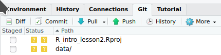
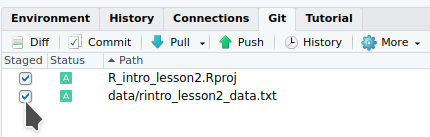
pwd (print working directory) in the Terminal shows you the directory you are currently in.TerminalYou don’t technically need to use Git and GitHub to code your data analysis. You could just store your files locally. BUT: I strongly recommend you make a Git repository for every data analysis project. It really helps to keep things organized in one place, not lose your code, go back to earlier versions, share it, collaborate on it, and so on. To practice, we will create a repository for every lesson.
We will now create a remote repository on Github, copy it to our local PCs, and then continue Lesson 2 in that local repository.
New on the top left.Your repositories or Repositories.As shown in the screenshot below:
Create repository: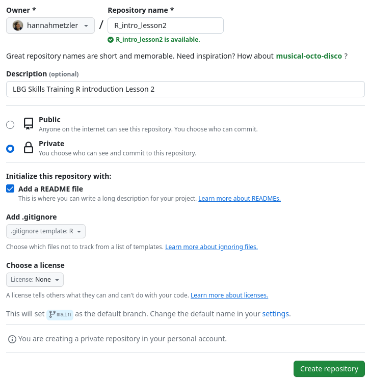
README.md: where you describe the project (folder structure, content, etc.).gitignore: Hidden file that tells Git what not to upload to GitHub (e.g., figures)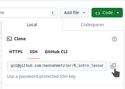
cd. (I want it in my folder AnalysisProjects)git clone and paste your repository link:
There is now a folder with the name of the remote repository in the directory you “cloned” it to. (For me, in the AnalysisProjects/ folder.) In that folder, let’s start our first R-project!
Create a project (or New Project in the File menu).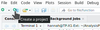
Existing DirectoryBrowse to navigate to our folder R_intro_lesson_2 and click Create Project
From now on, you can double click this Rproject file in your R_intro_lesson2 folder to directly open Rstudio from this folder.
We can now back up the project and data to a “remote repository” on GitHub.
We will finally start coding!
File (top left)rintro_lesson2Ctrl+Shift+C / Cmd+Shift+CCtrl + EnterCtrl + Shift + EnterWrite and run the code below:
## LOAD PACKAGES ####
library(tidyverse)read_csv() from the package readr.## READ IN DATA AND ORGANIZE ####
# Read in data
data = readr::read_csv("data/pets.csv", col_types = "cffiid")"data/pets.csv"col_types = "cffiid" defines the type of variable - we will get to this below.The first and last rows of the data frame:
| id | pet | country | score | age | weight |
|---|---|---|---|---|---|
| S001 | dog | UK | 90 | 6 | 19.78932 |
| S002 | dog | UK | 107 | 8 | 20.01422 |
| S003 | dog | UK | 94 | 2 | 19.14863 |
| S004 | dog | UK | 120 | 10 | 19.56953 |
| S005 | dog | UK | 111 | 4 | 21.39259 |
| S006 | dog | UK | 110 | 8 | 21.31880 |
| id | pet | country | score | age | weight |
|---|---|---|---|---|---|
| S795 | ferret | NL | 116 | 1 | 3.0276944 |
| S796 | ferret | NL | 118 | 7 | 3.2127433 |
| S797 | ferret | NL | 98 | 10 | 0.7909462 |
| S798 | ferret | NL | 123 | 3 | 3.9612231 |
| S799 | ferret | NL | 103 | 8 | 6.9195795 |
| S800 | ferret | NL | 120 | 5 | 0.5048159 |
data is our data frame (the whole data table with variables as columns and observations as rows)id, pet, score, age, weight are variablesdog and ferret are levels of the variable petUK and NL are levels of the variable countryNow, we’ll have a look at the data using these functions (from basic R):
Write and then run the code below. After each written line, use Ctrl + Enter to run it.
# Look at data
dim(data)
head(data)
tail(data)
xtabs(~pet, data)
All of this is basic R. In addition, we can use functions from packages. Using glimpse() from dplyr gives you an overview of the data:
dplyr::glimpse(data)Rows: 800
Columns: 6
$ id <chr> "S001", "S002", "S003", "S004", "S005", "S006", "S007", "S008"…
$ pet <fct> dog, dog, dog, dog, dog, dog, dog, dog, dog, dog, dog, dog, do…
$ country <fct> UK, UK, UK, UK, UK, UK, UK, UK, UK, UK, UK, UK, UK, UK, UK, UK…
$ score <int> 90, 107, 94, 120, 111, 110, 100, 107, 106, 109, 85, 110, 102, …
$ age <int> 6, 8, 2, 10, 4, 8, 9, 8, 6, 11, 5, 9, 1, 10, 7, 8, 1, 8, 5, 13…
$ weight <dbl> 19.78932, 20.01422, 19.14863, 19.56953, 21.39259, 21.31880, 19…Here, you can see that the data frame contains different types of variables:
chr (character): for variables with text (can contain any character: letter, numbers, symbols, spaces)fct(factor): for categorical variablesint (integer): numeric, stores whole numbersdbl (double): numeric, numbers with decimalsThere are always lots of ways to do the same thing in R.
Let’s say we want to create a new data frame that contains only cats data. Here are some ways to do that, which all produce exactly the same result. (Just examples, no need to understand this yet):
# basic R to extract specific rows from a dataframe
data_cats = data[data$pet == 'cat',]

# the function subset
data_cats = subset(data, pet == 'cat')

# using the function filter from the package dplyr
data_cats = data %>%
  dplyr::filter(pet == 'cat')
We’ll use dplyr (the third way). dplyr is a package from the Tidyverse for
# Select only cats
data_cats <- data %>%
  dplyr::filter(pet == "cat")
Here is a step by step explanation:
data_cats: new data frame<- (or =) is used to assigndata: original data frame%>% (or \|\>)\: a “pipe” in dplyr - let’s R know you are not done writing code, it waits until it gets a line not ending with %>% before executing the code.filter( ): verbpet: variablecat: level of the variable== is a marker of relationship (like <, >)You can use these keyboard shortcuts:
<- for assigning: Alt + - or Option + -%>% pipe: Shift + Ctrl + M or Cmd + Shift + MLet’s look at the top rows:
head(data_cats)| id | pet | country | score | age | weight |
|---|---|---|---|---|---|
| S401 | cat | UK | 95 | 2 | 8.571053 |
| S402 | cat | UK | 96 | 7 | 11.196836 |
| S403 | cat | UK | 72 | 4 | 10.307364 |
| S404 | cat | UK | 99 | 6 | 7.243529 |
| S405 | cat | UK | 85 | 3 | 6.650295 |
| S406 | cat | UK | 115 | 2 | 3.616348 |
There are only rows with cats left.
Look at the new data frame data_cats with all the functions you used above for data.
We’ll make a box plot showing the weight of the different pets. ggplot2 is a package from the Tidyverse that is very flexible for making pretty plots.
Plots in ggplot are created by adding elements on top of each other. See the vignette: We will use data, mapping and a layer for a box plot for now.
vignette("ggplot2")Start again with a section header (####).
## MAKE FIGURES ####
# Weight by pet
data.plot <- ggplot(data, aes(x = pet, y = weight)) +
  geom_boxplot()
data.plot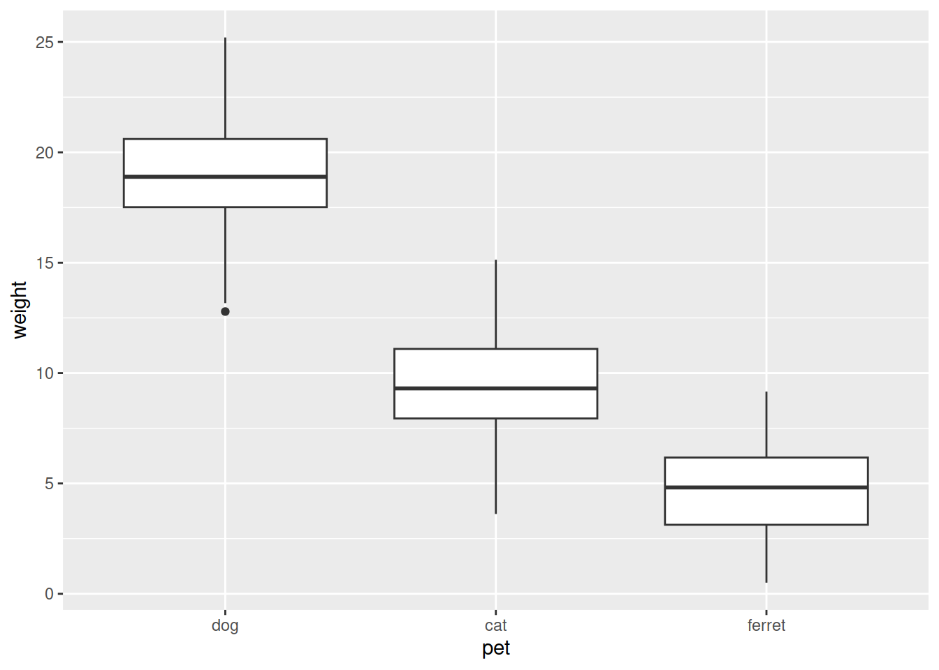
Step by step explanations:
ggplot()data)aes()) of the figure: here only which variable onto the x- and y-axis.+ to connect lines (like %>% above for dplyr)geom_ plus the type of plot, so here geom_boxplot.data.plot.data.plot to see the plot.It is very easy to make this plot pretty. With the code below:
fill = pet in the aesthetics.theme_bw()ggtitle()# Pretty plot
data.plot <- ggplot(data, aes(x = pet, y = weight, fill = pet)) +
geom_boxplot()+
theme_bw()+
ggtitle("Weight by pet")
data.plot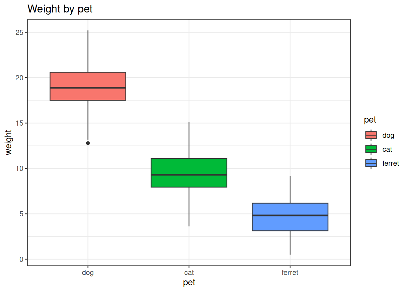
To save the plot to a file to use in your paper, use ggsave to save it in our subfolder for figures:
# save the plot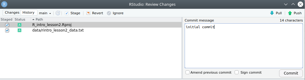
ggsave('figures/boxplot_pets_weight.png', plot = data.plot, width = 6, height = 4, dpi = 300)figures/ folder.CommitCommit to store a new version of your project, then Close.Push.write_up folder, naming them lesson2_environment.
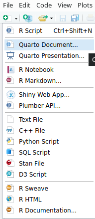
Create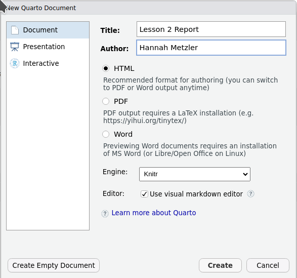
Save the Quarto document in your write_up folder Lesson2_Report
You can see that your R-script ends with .R, the Quarto file with .qmd
By clicking on Source, you will see the content written in “Markdown” language.
Markdown is
Let’s start writing in our Quarto Document:
Ctrl+Alt+I to insert a code chunk. ```{r} ` lets R know that the following is code.load("lesson2_environment.RData")# Data
Here is a look at our two data frames. First is the one we read in, the second is our subset with just the cat's data.
# Figure
Here's a figure of the weight of different pets in the dataset.Ctrl+Alt+I to insert them in the right places.head(data) and head(data_cats) to present your data sets under # Data.data.plot) under # Figure.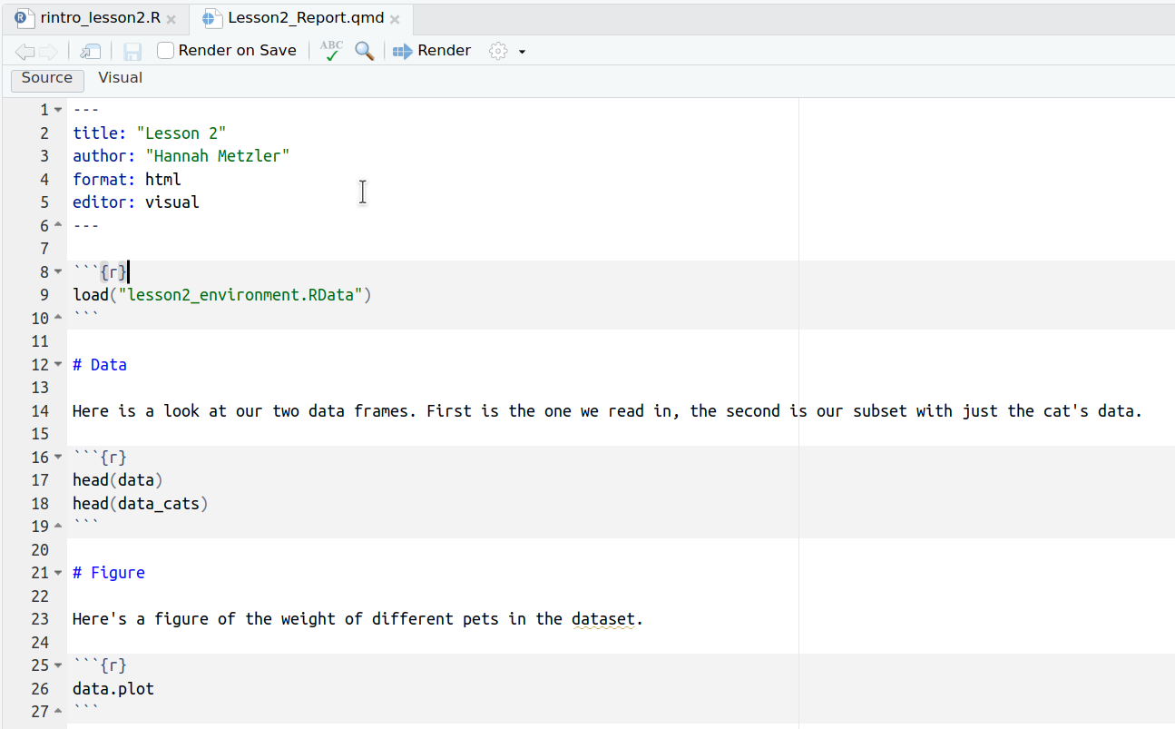
format: docx at the top, then render again as a Word document.quarto install tinytexYou can write a lot of your code directly in Quarto Documents, allowing to combine your results (tables, figures) with interpretations directly in the same document. Lead through your entire analyses step by step. If a step needs a lot of code, move that code to a script in the code folder, and call the script from your Quarto document using the function source(). For example, you could first call a script that cleans the data, then make figures and run statistical tests directly in the Quarto Document.
This lesson is based on:
Page Piccinini, R-Course, Lesson 1: R Basics.
Chapter 2 of: Lisa DeBruine & Dale Barr. (2022). Data Skills for Reproducible Research: (3.0) Zenodo. doi:10.5281/zenodo.6527194.