Lesson 3 extension: Data wrangling, t-tests and ANOVA
Course website: https://hannahmetzler.eu/R_intro/
Author
Hannah Metzler
Published
February 20, 2025
1 Project for extension of lesson 3: Comparison of baby names in Austria and the US
What about baby names in Austria?
Below, we read in data from Austria, make it comparable to the US data set, and then run a t-test to compare the popularity of baby names in the two countries.
2 Reading in and looking at data
2.1 Data from Austria
I downloaded data about given names in Austria from 1984 to 2022 from data.bv.at. Download the first file from there and put it into your data folder.
Continue working in your cleaning script from lesson 3, in the # READ DATA #### section.
To read the Austrian data, try the function read_csv(). Add after the lines that read in the data from the USA.
Here, I load the baby names data set, a default package included in the library “babynames”. To run the code below, you first need to install the package (via the console), and then load it by adding library(babynames) in your section for loading packages. This dataset, as opposed to the smaller one we used in lesson 3, includes all given names in the US, not just the ones from our course participants. Assign the dataset to data_usa.
# load the datasetdata(babynames)# assign it to data_usadata_usa = babynames
3 Get an overview of the dataset
To get an overview of this new data set, you could use any of the following functions:
summary() shows us that the earliest year in the data is 1984, the latest one 2022.
It also shows us that the column “Geschlecht” (sex) is not yet coded as a categorical variable.
summary(data_aut)
    C-JAHR-0    C-WOHNBEZIRK-0 C-GESCHLECHT-0  F-VORNAME_NORMALISIERT
 Min.   :1984   Min.   :101    Min.   :1.000   Length:1265460
 1st Qu.:1996   1st Qu.:319    1st Qu.:1.000   Class :character
 Median :2007   Median :506    Median :2.000   Mode  :character
 Mean   :2005   Mean   :563    Mean   :1.535
 3rd Qu.:2015   3rd Qu.:804    3rd Qu.:2.000
 Max.   :2022   Max.   :923    Max.   :2.000
 F-ANZAHL_LGEB
 Min.   : 1.00
 1st Qu.: 1.00
 Median : 1.00
 Mean   : 2.36
 3rd Qu.: 2.00
 Max.   :76.00
The function View() opens the data in an extra window.
View(data_aut)
The function str() shows you the structure of the data set.
If we compare the US and the Austrian data set, we can see that they cover different time spans.
summary(data_usa)
      year          sex                name                 n
 Min.   :1880   Length:1924665     Length:1924665     Min.   :    5.0
 1st Qu.:1951   Class :character   Class :character   1st Qu.:    7.0
 Median :1985   Mode  :character   Mode  :character   Median :   12.0
 Mean   :1975                                         Mean   :  180.9
 3rd Qu.:2003                                         3rd Qu.:   32.0
 Max.   :2017                                         Max.   :99686.0
      prop
 Min.   :2.260e-06
 1st Qu.:3.870e-06
 Median :7.300e-06
 Mean   :1.363e-04
 3rd Qu.:2.288e-05
 Max.   :8.155e-02
summary(data_aut_clean)
      year      living_district      sex            name
 Min.   :1984   Min.   :101     Min.   :1.000   Length:1265460
 1st Qu.:1996   1st Qu.:319     1st Qu.:1.000   Class :character
 Median :2007   Median :506     Median :2.000   Mode  :character
 Mean   :2005   Mean   :563     Mean   :1.535
 3rd Qu.:2015   3rd Qu.:804     3rd Qu.:2.000
 Max.   :2022   Max.   :923     Max.   :2.000
       n
 Min.   : 1.00
 1st Qu.: 1.00
 Median : 1.00
 Mean   : 2.36
 3rd Qu.: 2.00
 Max.   :76.00
Let’s keep only years we have in both datasets. First, filtering the Austrian dataset:
data_aut_clean <- data_aut %>% dplyr::rename(year ='C-JAHR-0', sex ='C-GESCHLECHT-0',living_district ='C-WOHNBEZIRK-0',name ='F-VORNAME_NORMALISIERT',n ='F-ANZAHL_LGEB') %>%#keep only years up to 2017filter(year <=2017)# Check the new data framesummary(data_aut_clean)
      year      living_district      sex            name
 Min.   :1984   Min.   :101     Min.   :1.000   Length:1047654
 1st Qu.:1994   1st Qu.:319     1st Qu.:1.000   Class :character
 Median :2004   Median :506     Median :2.000   Mode  :character
 Mean   :2002   Mean   :560     Mean   :1.541
 3rd Qu.:2011   3rd Qu.:804     3rd Qu.:2.000
 Max.   :2017   Max.   :923     Max.   :2.000
       n
 Min.   : 1.000
 1st Qu.: 1.000
 Median : 1.000
 Mean   : 2.458
 3rd Qu.: 2.000
 Max.   :76.000
Next, filter out all years before 1984 from the USA data set:
data_usa_clean = data_usa %>%#keep only years from 1984 onfilter(year >1983)summary(data_usa_clean)
      year          sex                name                 n
 Min.   :1984   Length:982833      Length:982833      Min.   :    5.0
 1st Qu.:1994   Class :character   Class :character   1st Qu.:    7.0
 Median :2003   Mode  :character   Mode  :character   Median :   11.0
 Mean   :2002                                         Mean   :  129.1
 3rd Qu.:2010                                         3rd Qu.:   29.0
 Max.   :2017                                         Max.   :67736.0
      prop
 Min.   :2.260e-06
 1st Qu.:3.290e-06
 Median :5.640e-06
 Mean   :6.431e-05
 3rd Qu.:1.438e-05
 Max.   :3.610e-02
4.3 Changing the format of columns
To run tests comparing both countries, we need to join both data frames into one. There are several steps to prepare our data sets for this.
First, columns in both data frames need the same format.
The US data had the following formats (see second column):
So, in the Austrian data, we need sex to be a character vector with levels “M” and “F” instead of “1” and “2”.
We will use the ifelse() function, within a mutate() call to transform the variable sex.
If you check the help for ?ifelse, the Usage section shows you how to use it: ifelse(test, yes, no).
The arguments for the ifelse() function start with a condition (rows where the column sex is equal to “1”), then specifies what happens if the condition is met (use the label “M”), and then lists what should happen otherwise/else (use the label “F”).
Now, add this as a last line to where you created data_aut_clean:
data_aut_clean <- data_aut %>% dplyr::rename(year ='C-JAHR-0', sex ='C-GESCHLECHT-0',living_district ='C-WOHNBEZIRK-0',name ='F-VORNAME_NORMALISIERT',n ='F-ANZAHL_LGEB') %>%#keep only years up to 2017filter(year <=2017) %>%# Recode the levels of sex from 1 and 2, to M and Fmutate(sex =ifelse(sex =="1", "M", "F"))# check if there is now F instead of 1, and M instead of M: glimpse(data_aut_clean)
Next, we need to tell statistics from Austria and the US apart, once they are in a joint data frame. Therefore, let’s add a variable that identifies the country.
We use rep() to repeat “Austria” n times, and set nrow() to the number of rows of the Austrian data.
data_aut_clean <- data_aut %>% dplyr::rename(year ='C-JAHR-0', sex ='C-GESCHLECHT-0',living_district ='C-WOHNBEZIRK-0',name ='F-VORNAME_NORMALISIERT',n ='F-ANZAHL_LGEB') %>%#keep only years up to 2017filter(year <=2017) %>%# Recode the levels of sex from 1 and 2, to M and Fmutate(sex =ifelse(sex =="1", "M", "F")) %>%#create a country variable for Austriamutate(country =rep("Austria", n=nrow(data_aut)))
Now, let’s repeat this step for the USA data. Just add a line to where you started to clean the US data:
data_usa_clean = data_usa %>%#keep only years from 1984 onfilter(year >1983) %>%#Create a country variable for the USmutate(country =rep("USA", n=nrow(babynames)))
4.5 Grouping data and summarising statistics
The US data did not separate names per living district.
To make our Austrian data similar, let’s group names across districts, so that we get the total number of names per year and sex.
Using group_by() first group the data by year, sex and name, because we want the total n for each of these combined categories.
We also add the column country, because we want to keep it, although it does not create any additional grouping.
We then summarise() the data by calculating the sum() of the number of names (n).
summarise() is similar to mutate(), but creates one line of output per group. Here, it collapses across districts, reducing the row number for each name.
mutate() creates as many lines of output as input.
Finally, we ungroup() the data again.
data_aut_clean <- data_aut %>%rename(year ='C-JAHR-0', sex ='C-GESCHLECHT-0',living_district ='C-WOHNBEZIRK-0',name ='F-VORNAME_NORMALISIERT',n ='F-ANZAHL_LGEB') %>%#keep only years up to 2017filter(year <=2017) %>%# Recode the levels of sex from 1 and 2, to M and Fmutate(sex =ifelse(sex =="1", "M", "F")) %>%#create a country variable for Austriamutate(country =rep("Austria", n=nrow(data_aut))) %>%#group by year, sex and name and calculate the new sum for each categorygroup_by(year, sex, name, country) %>%summarise(n =sum(n)) %>%ungroup()
Finally, we also want to calculate the proportion variable that exists in the US data set (propotion of babies getting each name).
N, the total number of babies, is obviously different because the US is larger.
Using the proportion allows us to meaningfully compare the popularity of names between countries.
We first want to calculate the sum of all babies born in each year (n_total), and then divide n of each name by the years’ total.
To calculate the sum per year, we again use group_by(), grouping only by year.
We again add country, also this does not create a group, to keep country variable.
data_aut_clean <- data_aut %>%rename(year ='C-JAHR-0', sex ='C-GESCHLECHT-0',living_district ='C-WOHNBEZIRK-0',name ='F-VORNAME_NORMALISIERT',n ='F-ANZAHL_LGEB') %>%#keep only years up to 2017filter(year <=2017) %>%# Recode the levels of sex from 1 and 2, to M and Fmutate(sex =ifelse(sex =="1", "M", "F")) %>%#create a country variable for Austriamutate(country =rep("Austria", n=nrow(data_aut))) %>%#group by year, sex and name and calculate the new sum for each categorygroup_by(year, sex, name, country) %>%summarise(n =sum(n)) %>%# see lesson 3 page for documentationungroup()%>%#calculate total number of birth per year, and then proportion for each name out of this totalgroup_by(year, country) %>%mutate(n_total =sum(n), prop = n/n_total) %>%ungroup()head(data_aut_clean)
year
sex
name
country
n
n_total
prop
1984
F
Abigail
Austria
1
83856
0.0000119
1984
F
Adele
Austria
2
83856
0.0000239
1984
F
Adelheid
Austria
23
83856
0.0002743
1984
F
Adina
Austria
2
83856
0.0000239
1984
F
Adriane
Austria
1
83856
0.0000119
1984
F
Agata
Austria
1
83856
0.0000119
4.6 Filter out one name
Once this is done, you can again filter one name. I recommend taking a name that occurs in both men and women (like “Kim”), so the results of the ANOVA below make more sense.
Add another filter() call to each of the data sets for this. After this, the cleaning and data organizing is finished.
Austrian data set complete data cleaning and organizing:
data_aut_clean <- data_aut %>%rename(year ='C-JAHR-0', sex ='C-GESCHLECHT-0',living_district ='C-WOHNBEZIRK-0',name ='F-VORNAME_NORMALISIERT',n ='F-ANZAHL_LGEB') %>%#keep only years up to 2017filter(year <=2017) %>%# Re-code the levels of sex from 1 and 2, to M and Fmutate(sex =ifelse(sex =="1", "M", "F")) %>%#create a country variable for Austriamutate(country =rep("Austria", n=nrow(data_aut))) %>%#group by year, sex and name and calculate the new sum for each categorygroup_by(year, sex, name, country) %>%summarise(n =sum(n)) %>%# see lesson 3 page for documentationungroup()%>%#calculate total number of birth per year, and then proportion for each name out of this totalgroup_by(year, country) %>%mutate(n_total =sum(n), prop = n/n_total) %>%ungroup() %>%#filter out your namefilter(name =="Kim")
USA data set complete data cleaning and organizing:
data_usa_clean = data_usa %>%#keep only years from 1984 onfilter(year >1983) %>%#Create a country variable for the USmutate(country =rep("USA", n=nrow(data_usa))) %>%#filter out your namefilter(name =="Kim")
Have a look at both organized data sets:
head(data_usa_clean)
year
sex
name
n
prop
country
1984
F
Kim
387
0.0002147
USA
1984
M
Kim
92
0.0000490
USA
1985
F
Kim
348
0.0001885
USA
1985
M
Kim
92
0.0000478
USA
1986
F
Kim
281
0.0001523
USA
1986
M
Kim
81
0.0000422
USA
head(data_aut_clean)
year
sex
name
country
n
n_total
prop
1984
F
Kim
Austria
1
83856
1.19e-05
1984
M
Kim
Austria
2
83856
2.39e-05
1985
F
Kim
Austria
3
82379
3.64e-05
1986
F
Kim
Austria
6
82056
7.31e-05
1987
F
Kim
Austria
2
81351
2.46e-05
1988
F
Kim
Austria
7
82545
8.48e-05
5 Combine two data frames
Now we can combine the 2 data frames. We’ll learn about dplyr verbs that work on two data frames. Until now, all verbs (filter, mutate, summarise, rename, recode) manipulated only one data frame.
We will use the function full_join: it
R looks for column they have in common
then looks for rows that have the same matching values
combines them into a new data frame, including all the other columns from both data frames
full_join() is one of 4 Mutating joins. It keeps all observations from both data frames.
Check out inner_join, right_join, and left_join with the Examples provided in the help on ?full_join when you have a moment. It takes a bit of time to understand them.
# join the two data frames, keeping all columns and entries from both data framesdata_combined <- data_usa_clean %>%full_join(data_aut_clean) head(data_combined)
year
sex
name
n
prop
country
n_total
1984
F
Kim
387
0.0002147
USA
NA
1984
M
Kim
92
0.0000490
USA
NA
1985
F
Kim
348
0.0001885
USA
NA
1985
M
Kim
92
0.0000478
USA
NA
1986
F
Kim
281
0.0001523
USA
NA
1986
M
Kim
81
0.0000422
USA
NA
To see data points from both countries, you could sort values by year using arrange().
In addition, lets transform the columns sex and country into categorical variables (factors).
data_combined <- data_usa_clean %>%# join the two data framesfull_join(data_aut_clean) %>%# sort by yeararrange(year)%>%# transform sex into a factormutate(sex =factor(sex)) %>%# transform country into a factor with 2 levels:mutate(country =factor(country))head(data_combined)
year
sex
name
n
prop
country
n_total
1984
F
Kim
387
0.0002147
USA
NA
1984
M
Kim
92
0.0000490
USA
NA
1984
F
Kim
1
0.0000119
Austria
83856
1984
M
Kim
2
0.0000239
Austria
83856
1985
F
Kim
348
0.0001885
USA
NA
1985
M
Kim
92
0.0000478
USA
NA
summary(data_combined)
      year      sex        name                 n               prop
 Min.   :1984   F:68   Length:127         Min.   :  1.00   Min.   :3.210e-06
 1st Qu.:1993   M:59   Class :character   1st Qu.:  7.00   1st Qu.:1.510e-05
 Median :2001          Mode  :character   Median : 18.00   Median :3.701e-05
 Mean   :2001                             Mean   : 50.66   Mean   :7.947e-05
 3rd Qu.:2009                             3rd Qu.: 70.50   3rd Qu.:1.295e-04
 Max.   :2017                             Max.   :387.00   Max.   :3.562e-04

    country      n_total
 Austria:59   Min.   :64431
 USA    :68   1st Qu.:67375
              Median :76058
              Mean   :74895
              3rd Qu.:82366
              Max.   :85333
              NA's   :68
You might want to drop the column n_total, which only has values for Austria. You can do this with select():
It selects the columns you list.
if you add a minus, it deletes the columns you list
data_combined <- data_usa_clean %>%# join the two data framesfull_join(data_aut_clean) %>%# sort by yeararrange(year)%>%# transform sex into a factormutate(sex =factor(sex)) %>%# transform country into a factor with 2 levels:mutate(country =factor(country)) %>%# delete the column n_totalselect(-n_total) #to delete multiple columns: -c("column_1", "column_2")data_combined
year
sex
name
n
prop
country
1984
F
Kim
387
0.0002147
USA
1984
M
Kim
92
0.0000490
USA
1984
F
Kim
1
0.0000119
Austria
1984
M
Kim
2
0.0000239
Austria
1985
F
Kim
348
0.0001885
USA
1985
M
Kim
92
0.0000478
USA
1985
F
Kim
3
0.0000364
Austria
1986
F
Kim
281
0.0001523
USA
1986
M
Kim
81
0.0000422
USA
1986
F
Kim
6
0.0000731
Austria
1987
F
Kim
280
0.0001494
USA
1987
M
Kim
76
0.0000390
USA
1987
F
Kim
2
0.0000246
Austria
1988
F
Kim
252
0.0001311
USA
1988
M
Kim
89
0.0000445
USA
1988
F
Kim
7
0.0000848
Austria
1989
F
Kim
259
0.0001300
USA
1989
M
Kim
72
0.0000344
USA
1989
F
Kim
15
0.0001818
Austria
1989
M
Kim
6
0.0000727
Austria
1990
F
Kim
257
0.0001251
USA
1990
M
Kim
66
0.0000307
USA
1990
F
Kim
12
0.0001441
Austria
1990
M
Kim
1
0.0000120
Austria
1991
F
Kim
207
0.0001018
USA
1991
M
Kim
60
0.0000283
USA
1991
F
Kim
20
0.0002348
Austria
1992
F
Kim
182
0.0000908
USA
1992
M
Kim
45
0.0000214
USA
1992
F
Kim
20
0.0002407
Austria
1992
M
Kim
1
0.0000120
Austria
1993
F
Kim
185
0.0000938
USA
1993
M
Kim
39
0.0000189
USA
1993
F
Kim
17
0.0002080
Austria
1994
F
Kim
160
0.0000821
USA
1994
M
Kim
46
0.0000226
USA
1994
F
Kim
20
0.0002526
Austria
1995
F
Kim
135
0.0000703
USA
1995
M
Kim
31
0.0000154
USA
1995
F
Kim
8
0.0001055
Austria
1995
M
Kim
2
0.0000264
Austria
1996
F
Kim
130
0.0000678
USA
1996
M
Kim
47
0.0000235
USA
1996
F
Kim
15
0.0001972
Austria
1996
M
Kim
2
0.0000263
Austria
1997
F
Kim
110
0.0000576
USA
1997
M
Kim
20
0.0000100
USA
1997
F
Kim
18
0.0002487
Austria
1997
M
Kim
1
0.0000138
Austria
1998
F
Kim
102
0.0000526
USA
1998
M
Kim
24
0.0000118
USA
1998
F
Kim
15
0.0002148
Austria
1998
M
Kim
1
0.0000143
Austria
1999
F
Kim
133
0.0000683
USA
1999
M
Kim
29
0.0000142
USA
1999
F
Kim
16
0.0002393
Austria
1999
M
Kim
2
0.0000299
Austria
2000
F
Kim
116
0.0000581
USA
2000
M
Kim
18
0.0000086
USA
2000
F
Kim
10
0.0001493
Austria
2000
M
Kim
2
0.0000299
Austria
2001
F
Kim
100
0.0000505
USA
2001
M
Kim
26
0.0000126
USA
2001
F
Kim
12
0.0001855
Austria
2001
M
Kim
1
0.0000155
Austria
2002
F
Kim
111
0.0000562
USA
2002
M
Kim
14
0.0000068
USA
2002
F
Kim
12
0.0001781
Austria
2002
M
Kim
2
0.0000297
Austria
2003
F
Kim
83
0.0000414
USA
2003
M
Kim
17
0.0000081
USA
2003
F
Kim
14
0.0002098
Austria
2003
M
Kim
4
0.0000600
Austria
2004
F
Kim
91
0.0000451
USA
2004
M
Kim
18
0.0000085
USA
2004
F
Kim
23
0.0003349
Austria
2004
M
Kim
1
0.0000146
Austria
2005
F
Kim
73
0.0000360
USA
2005
M
Kim
13
0.0000061
USA
2005
F
Kim
14
0.0002070
Austria
2005
M
Kim
1
0.0000148
Austria
2006
F
Kim
85
0.0000407
USA
2006
M
Kim
10
0.0000046
USA
2006
F
Kim
24
0.0003562
Austria
2006
M
Kim
2
0.0000297
Austria
2007
F
Kim
104
0.0000492
USA
2007
M
Kim
10
0.0000045
USA
2007
F
Kim
23
0.0003504
Austria
2007
M
Kim
2
0.0000305
Austria
2008
F
Kim
63
0.0000303
USA
2008
M
Kim
7
0.0000032
USA
2008
F
Kim
21
0.0003161
Austria
2008
M
Kim
5
0.0000753
Austria
2009
F
Kim
48
0.0000237
USA
2009
M
Kim
17
0.0000080
USA
2009
F
Kim
14
0.0002173
Austria
2009
M
Kim
1
0.0000155
Austria
2010
F
Kim
52
0.0000266
USA
2010
M
Kim
9
0.0000044
USA
2010
F
Kim
15
0.0001946
Austria
2010
M
Kim
1
0.0000130
Austria
2011
F
Kim
50
0.0000258
USA
2011
M
Kim
7
0.0000034
USA
2011
F
Kim
21
0.0002746
Austria
2011
M
Kim
1
0.0000131
Austria
2012
F
Kim
91
0.0000470
USA
2012
M
Kim
9
0.0000044
USA
2012
F
Kim
19
0.0002458
Austria
2012
M
Kim
2
0.0000259
Austria
2013
F
Kim
62
0.0000322
USA
2013
M
Kim
8
0.0000040
USA
2013
F
Kim
14
0.0001802
Austria
2014
F
Kim
69
0.0000354
USA
2014
M
Kim
19
0.0000093
USA
2014
F
Kim
17
0.0002128
Austria
2015
F
Kim
72
0.0000370
USA
2015
M
Kim
11
0.0000054
USA
2015
F
Kim
11
0.0001336
Austria
2015
M
Kim
2
0.0000243
Austria
2016
F
Kim
52
0.0000270
USA
2016
M
Kim
7
0.0000035
USA
2016
F
Kim
11
0.0001290
Austria
2016
M
Kim
1
0.0000117
Austria
2017
F
Kim
46
0.0000245
USA
2017
M
Kim
8
0.0000041
USA
2017
F
Kim
4
0.0000469
Austria
2017
M
Kim
1
0.0000117
Austria
6 Figures script
In the figures script, add the following figure:
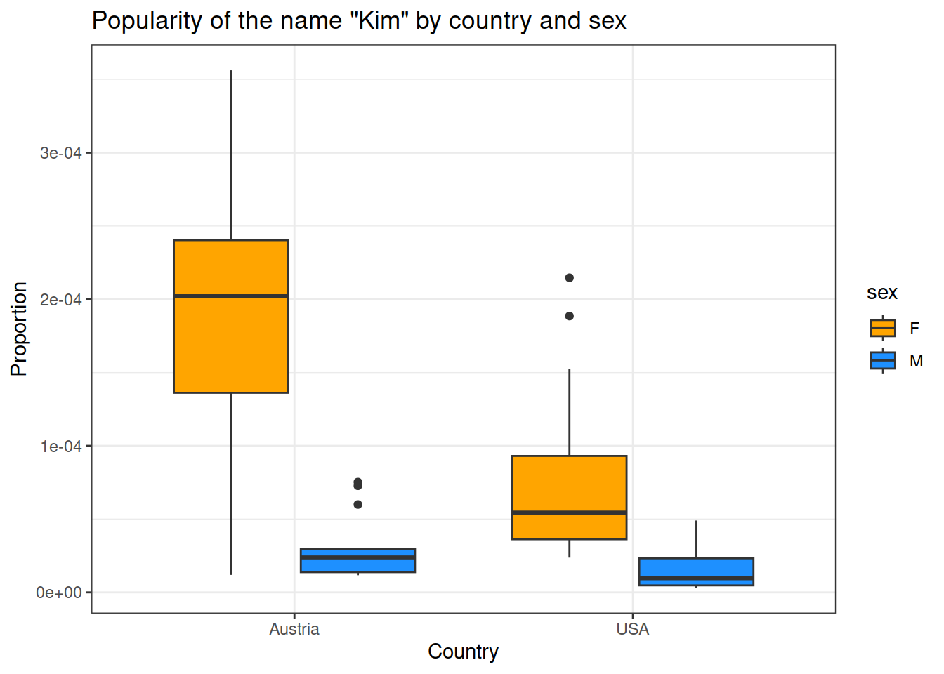
# Boxplot of name propotion by sex and countryggplot(data_combined, aes(country, prop, fill = sex)) +geom_boxplot() +scale_fill_manual(values =c("orange", "dodgerblue")) +labs(x ="Country", y ="Proportion") +theme(text =element_text(size =20, family ="Times"))+theme_bw()+ggtitle("Popularity of the name \"Kim\" by country and sex")
Figure 1. Scores by pet type and country.
In both countries, there are more women than men with the name Kim (main effect of sex).
There is also a main effect of country: in the USA, the name “Kim” is less popular than in Austria.
In addition, there is an interaction: The difference in women named “Kim” between the two countries is larger than the difference for men.
7 Statistics script
In the statistics script, rerun the line with source() to read in the new data from the cleaning script.
7.1 T-test by country
Is your name more popular in Austria or the USA? Although this data is not normally distributed, I want to show you how to do a t-test:
# t-test between countriest.test(prop ~ country, data = data_combined)
    Welch Two Sample t-test

data:  prop by country
t = 5.0499, df = 76.579, p-value = 2.914e-06
alternative hypothesis: true difference in means between group Austria and group USA is not equal to 0
95 percent confidence interval:
 4.558866e-05 1.049556e-04
sample estimates:
mean in group Austria     mean in group USA
         1.197764e-04          4.450426e-05
You can see that “Kim” is significantly more popular in Austria compared to the US.
# t-test between men and woment.test(prop ~ sex, data = data_combined)
    Welch Two Sample t-test

data:  prop by sex
t = 9.6265, df = 71.905, p-value = 1.458e-14
alternative hypothesis: true difference in means between group F and group M is not equal to 0
95 percent confidence interval:
 8.733425e-05 1.329523e-04
sample estimates:
mean in group F mean in group M
   1.306421e-04    2.049884e-05
You can see that “Kim” is much more frequent in women than men.
7.2 Multi-factorial ANOVA: Difference in name popularity by sex and country
If you want to investigate if your name is more popular for men or women, and if this difference varies across countries, you could run an ANOVA (analysis of variance) with two factors (sex and country).
I recommend using the package “ez” for this. Load it at the top of your statistics script.
# Install in the consoleinstall.packages("ez")# In your script: library(ez)
After your other analyses (the linear regression and t-test), you can now add the ANOVA in your statistics script, using the function ezANOVA(). It’s arguments:
the data frame
dv: the dependent variable (proportion)
wid: the columns that identify unique rows in your data frame. Here these are 2 columns: each name exists for each year. The function ezANOVA requires that you enter multiple columns as a list: .("column 1", "column 2").
A list in R is a very flexible object type that can store all kinds of objects of different dimensions. The first object could be a string, the second a data frame, the third a vector.
between: the predictors. ezANOVA requires that you enter multiple predictors as a list: .(x, y, z)
Type 3 defines which sum of squares are calculated for the ANOVA. This is detailed statistics knowledge, and only slightly changes your result. In any case, SPSS by default gives you type 3, so we use it here.
$ANOVA
       Effect DFn DFd         F            p p<.05       ges
2     country   1 123  42.13132 1.886914e-09     * 0.2551383
3         sex   1 123 127.77207 9.391571e-21     * 0.5095148
4 country:sex   1 123  30.59984 1.817898e-07     * 0.1992179

$`Levene's Test for Homogeneity of Variance`
  DFn DFd          SSn          SSd        F           p p<.05
1   3 123 6.930065e-08 1.709389e-07 16.62188 3.96263e-09     *
7.3 Make a table with statistics and export it to a csv-file
# Create a table with number of babyes with the name Kim per country and sex, with mean and sd: summary_table <- data_combined %>%group_by(country, sex) %>%#summarise: calculate one number/statistic per group created abovesummarise(n =n(), # calculate mean and standard deviationmean_proportion =mean(prop), sd_proportion =sd(prop), # transform to percent for readibilitymean_percent = mean_proportion*100, sd_percent = sd_proportion*100 ) %>%ungroup()# printsummary_table
country
sex
n
mean_proportion
sd_proportion
mean_percent
sd_percent
Austria
F
34
0.0001888
8.94e-05
0.0188840
0.0089409
Austria
M
25
0.0000259
1.80e-05
0.0025850
0.0017965
USA
F
34
0.0000724
4.96e-05
0.0072444
0.0049594
USA
M
34
0.0000166
1.45e-05
0.0016564
0.0014458
# To write results to an excel table, in order to include tables into papers, for example:
readr::write_csv(summary_table, 'write_up/descriptives_table.csv')
8 Transforming data from long to wide format
In this section, you’ll learn about a few functions that you will regularly need - although we did not need them for the analyses above.
Sometimes you need your data in a wide format, that is, multiple columns for the dependent variable, as here separate columns for Austria and the US and this for each sex.
SPSS and other statistics software need data in this format by default.
In R, you can change the format of the data frame using the function pivot_wider() from the tidyverse package tidyr.
Install the package, and load the library at the start of your statistics script.
Arguments of pivot_wider():
the data frame
id_cols: the column or columns that identify a single unique row in your data frame. This could be you participant ID. Here, it is each name per year.
names_from: the variables for which you want to create new columns (or column/variable names)
values_from: the value/variable you want to fill these columns with, here proportion (log transformed)
Write the following code in your section for organizing data in the statistics script.
## ORGANIZE DATA ##### create data frame in wide formatdata_combined_wide = tidyr::pivot_wider(data_combined, id_cols =c("year", "name"), names_from =c("country", "sex"), values_from ="prop")head(data_combined_wide)
year
name
USA_F
USA_M
Austria_F
Austria_M
1984
Kim
0.0002147
4.90e-05
0.0000119
2.39e-05
1985
Kim
0.0001885
4.78e-05
0.0000364
NA
1986
Kim
0.0001523
4.22e-05
0.0000731
NA
1987
Kim
0.0001494
3.90e-05
0.0000246
NA
1988
Kim
0.0001311
4.45e-05
0.0000848
NA
1989
Kim
0.0001300
3.44e-05
0.0001818
7.27e-05
This will create an extra column per country and gender (4 columns in total)
The function that transforms data frames in the reverse direction, is called pivot_longer(). Try to back transform your wide data frame to a long one as an exercise!
You can see that the wide data frame has empty values (NA = not available) for men in the USA. our pivot_wider call added a row for each year where the name Kim occurred in any country or sex, this is why cells with no data for Kim now have an NA.You could also check how many NAs are in the column with the line of code below.
# are there any missing values? How many?sum(is.na(data_combined_wide$Austria_M))
[1] 9
We actually know that in this case, NA simply means there were no babies with that name. So let’s replace the NAs with 0 using ifelse(). It’s arguments:
The condition for if is that Austria_M is an NA, you can check this with the function is.na() which will give TRUE for missing values (NAs).
if this condition is met (TRUE), then replace with a 0
else, keep the value of Austria_M.
data_combined_wide = data_combined_wide %>%# replace NAs with zeromutate(Austria_M =ifelse(is.na(Austria_M), 0, Austria_M))data_combined_wide
year
name
USA_F
USA_M
Austria_F
Austria_M
1984
Kim
0.0002147
4.90e-05
0.0000119
2.39e-05
1985
Kim
0.0001885
4.78e-05
0.0000364
0.00e+00
1986
Kim
0.0001523
4.22e-05
0.0000731
0.00e+00
1987
Kim
0.0001494
3.90e-05
0.0000246
0.00e+00
1988
Kim
0.0001311
4.45e-05
0.0000848
0.00e+00
1989
Kim
0.0001300
3.44e-05
0.0001818
7.27e-05
1990
Kim
0.0001251
3.07e-05
0.0001441
1.20e-05
1991
Kim
0.0001018
2.83e-05
0.0002348
0.00e+00
1992
Kim
0.0000908
2.14e-05
0.0002407
1.20e-05
1993
Kim
0.0000938
1.89e-05
0.0002080
0.00e+00
1994
Kim
0.0000821
2.26e-05
0.0002526
0.00e+00
1995
Kim
0.0000703
1.54e-05
0.0001055
2.64e-05
1996
Kim
0.0000678
2.35e-05
0.0001972
2.63e-05
1997
Kim
0.0000576
1.00e-05
0.0002487
1.38e-05
1998
Kim
0.0000526
1.18e-05
0.0002148
1.43e-05
1999
Kim
0.0000683
1.42e-05
0.0002393
2.99e-05
2000
Kim
0.0000581
8.60e-06
0.0001493
2.99e-05
2001
Kim
0.0000505
1.26e-05
0.0001855
1.55e-05
2002
Kim
0.0000562
6.80e-06
0.0001781
2.97e-05
2003
Kim
0.0000414
8.10e-06
0.0002098
6.00e-05
2004
Kim
0.0000451
8.50e-06
0.0003349
1.46e-05
2005
Kim
0.0000360
6.10e-06
0.0002070
1.48e-05
2006
Kim
0.0000407
4.60e-06
0.0003562
2.97e-05
2007
Kim
0.0000492
4.50e-06
0.0003504
3.05e-05
2008
Kim
0.0000303
3.20e-06
0.0003161
7.53e-05
2009
Kim
0.0000237
8.00e-06
0.0002173
1.55e-05
2010
Kim
0.0000266
4.40e-06
0.0001946
1.30e-05
2011
Kim
0.0000258
3.40e-06
0.0002746
1.31e-05
2012
Kim
0.0000470
4.40e-06
0.0002458
2.59e-05
2013
Kim
0.0000322
4.00e-06
0.0001802
0.00e+00
2014
Kim
0.0000354
9.30e-06
0.0002128
0.00e+00
2015
Kim
0.0000370
5.40e-06
0.0001336
2.43e-05
2016
Kim
0.0000270
3.50e-06
0.0001290
1.17e-05
2017
Kim
0.0000245
4.10e-06
0.0000469
1.17e-05
9 Feedback welcome!
If you find any errors or things that are not explained in enough detail in this lesson, please let me know: metzler[@]csh.ac.at.